ModelsEnvironments  Explore with Other DoEs
Explore with Other DoEs
Design of Experiments (DoE) is the art of setting up an experimentation. In a model simulation context,
it boils down to declare the inputs under study (most of the time, they're parameters) and the values they will take, for a batch of several simulations, with the idea of revealing a property of the model (e.g. sensitivity).
Even if there are several state-of-the-art DoE methods implemented in OpenMOLE, we recommend to focus on OpenMOLE
new methods: PSE, and Calibration and Profiles which have been thought to improve the drawbacks of the classical methods.
Your model inputs can be sampled in the traditional way, by using grid (or regular) sampling, by sampling uniformly inside their domain.
For higher dimension input space, specific statistics techniques like Latin Hypercube Sampling and SobolSequence are available.
If you want to use design of experiments of your own you may also want to provide a csv file with your samples to OpenMOLE.
By defining your own exploration task on several types of input, you will be able to highlight some of your model inner properties like those revealed by sensitivity analysis, as shown in a toy example on a real world example
For a reasonable number of dimension and discretisation quanta (steps) values, complete sampling (or grid sampling) consists in producing every combination of the inputs possibles values, given their bounds and quanta of discretisation.
Method scores:
Regular sampling or Uniform Sampling are quite good for a first Input Space exploration when you don't know anything about its structure yet. Since it samples from the input space, the collected values from the model executions will reveal the output values obtained for "evenly spaced" inputs. Sure it's not perfect, but still , it gives a little bit of insights about model sensitivity (as input values vary within their domain) and if the output are fitness, it may present a little bit of optimization information (as the zone in which the fitness could be minimized).
The sampling does not reveal anything about the output space structure, as there is no reason than evenly spaced inputs lead to evenly spaced outputs. Basic sampling is hampered by input space dimensionality as high dimension spaces need a lot of samples to be covered, as well as a lot of memory to store them.
Complete sampling is declared as an ExplorationTask, where the bounds and discretisation quantum of each input to vary are declared using the following syntax :
Sampling can also be performed via a
The cartesian product operator can handle different data types :
The UniformDistribution[T]() take 10 is a uniform sampling of 10 numbers of the Long type, taken in the [Long.MIN_VALUE; Long.MAX_VALUE] domain of the Long native type.
Files are explored as items of a list. The items are gathered by the
If your input is one file among many, or a line among a CSV file, use the CSVSampling task and FileSampling task
Eventually, let's have a look at the stochasticity of the model. Looking at the plot, we see that there is a lot of variation possible, especially in the transition zone, around 60% density. Let's make a final exploration Task to investigate the variation of model outputs for several replications of the same parameterization. We now take densities within [50;70] and take 100 replications for each:
We obtain the following results, displayed as boxplots every percent (but results are obtained for every 0.1% density) to emphasize on the variations.

As we can see, stochasticity has an high effect right in the middle of the transition of regime, reaching maximum at 54%. Another interesting thing to investigate what would be the density from which the fire propagates to the end of the zone (right side of NetLogo World). A slight modification of the model code would do the trick (hint:
Your model inputs can be sampled in the traditional way, by using grid (or regular) sampling, by sampling uniformly inside their domain.
For higher dimension input space, specific statistics techniques like Latin Hypercube Sampling and SobolSequence are available.
If you want to use design of experiments of your own you may also want to provide a csv file with your samples to OpenMOLE.
By defining your own exploration task on several types of input, you will be able to highlight some of your model inner properties like those revealed by sensitivity analysis, as shown in a toy example on a real world example
For a reasonable number of dimension and discretisation quanta (steps) values, complete sampling (or grid sampling) consists in producing every combination of the inputs possibles values, given their bounds and quanta of discretisation.
Method scores:
Regular sampling or Uniform Sampling are quite good for a first Input Space exploration when you don't know anything about its structure yet. Since it samples from the input space, the collected values from the model executions will reveal the output values obtained for "evenly spaced" inputs. Sure it's not perfect, but still , it gives a little bit of insights about model sensitivity (as input values vary within their domain) and if the output are fitness, it may present a little bit of optimization information (as the zone in which the fitness could be minimized).
The sampling does not reveal anything about the output space structure, as there is no reason than evenly spaced inputs lead to evenly spaced outputs. Basic sampling is hampered by input space dimensionality as high dimension spaces need a lot of samples to be covered, as well as a lot of memory to store them.
Complete sampling is declared as an ExplorationTask, where the bounds and discretisation quantum of each input to vary are declared using the following syntax :
val input_i = Val[Int]
val input_j = Val[Double]

val exploration =
  ExplorationTask (
    (input_i in (0 to 10 by 2)) x
    (input_j in (0.0 to 5.0 by 0.5))
)Sampling can also be performed via a
UniformDistribution(maximum), that generates values uniformly
distributed between zero and the maximum provided argument.
Custom domains can be defined using transformations, as in the example below that generates values between -10 and + 10.
val my_input = Val[Double]
val exploration = ExplorationTask(
    (my_input in (UniformDistribution[Double](max=20) take 100)).map(x => x -10)
)
You can inject your own sampling in OpenMOLE through a CSV file. Considering a CSV file like:
In this example the column i in the CSV file is mapped to the variable i of OpenMOLE. The column name colD is mapped to the variable d. The column named colFileName is appended to the base directory "/path/of/the/base/dir/" and used as a file in OpenMOLE. As a sampling, the CSVSampling can directly be injected in an ExplorationTask. It will generate a different task for each entry in the file.
coldD,  colFileName,    i
0.7,    fic1,           8
0.9,    fic2,           19
0.8,    fic2,           19
val i = Val[Int]
val d = Val[Double]
val f = Val[File]

//Only comma separated files with header are supported for now
val s = CSVSampling("/path/to/a/file.csv") set (
  columns += i,
  columns += ("colD", d),
  fileColumns += ("colFileName", "/path/of/the/base/dir/", f),
  // comma ',' is the default separator, but you can specify a different one using
  separator := ','
)

val exploration = ExplorationTask(s)
In this example the column i in the CSV file is mapped to the variable i of OpenMOLE. The column name colD is mapped to the variable d. The column named colFileName is appended to the base directory "/path/of/the/base/dir/" and used as a file in OpenMOLE. As a sampling, the CSVSampling can directly be injected in an ExplorationTask. It will generate a different task for each entry in the file.
High dimension spaces must be handled via specific methods of the literature, because otherwise cartesian product
would be too memory consuming .
OpenMOLE includes two of these methods: Sobol Sequence
and Latin Hypercube Sampling , defined as specifications of the
Method scores:
These two methods perform allright in terms of Input Space Exploration (which is normal as they were built for that extent), anyhow, they are superior to uniform sampling or grid sampling, but share the same intrinsic limitations. There is no special way of handling Stochasticity of the model, out of standard replications.
These methods are not expansive per se , it depends on the magnitude of the Input Space you want to be covered.
ExplorationTask:
Method scores:
These two methods perform allright in terms of Input Space Exploration (which is normal as they were built for that extent), anyhow, they are superior to uniform sampling or grid sampling, but share the same intrinsic limitations. There is no special way of handling Stochasticity of the model, out of standard replications.
These methods are not expansive per se , it depends on the magnitude of the Input Space you want to be covered.
Latin Hypercube Sampling
val i = Val[Double]
val j = Val[Double]

val my_LHS_sampling =
  ExplorationTask (
    LHS(
      100, // Number of points of the LHS
      i in Range(0.0, 10.0),
      j in Range(0.0, 5.0)
    )
  )
Sobol Sequence
val i = Val[Double]
val j = Val[Double]

val my_sobol_sampling =
  ExplorationTask (
    SobolSampling(
      100, // Number of points
      i in Range(0.0, 10.0),
      j in Range(0.0, 5.0)
    )
  )
Exploration can be performed on several inputs domains, using the cartesian product operator: x.
The basic syntax to explore 2 inputs (i.e. every combination of 2 inputs values) isval i = Val[Int]
val j = Val[Double]
val exploration =
ExplorationTask (
(i in (0 to 10 by 2)) x
(j in (0.0 to 5.0 by 0.5))
)Different Types of inputs
The cartesian product operator can handle different data types :
val i = Val[Int]
val j = Val[Double]
val k = Val[String]
val l = Val[Long]
val m = Val[File]

val exploration =
  ExplorationTask (
    (i in (0 to 10 by 2)) x
    (j in (0.0 to 5.0 by 0.5)) x
    (k in List("Leonardo", "Donatello", "Raphaël", "Michelangelo")) x
    (l in (UniformDistribution[Long]() take 10)) x
    (m in (workDirectory / "dir").files().filter(f => f.getName.startsWith("exp") && f.getName.endsWith(".csv")))
  )
The UniformDistribution[T]() take 10 is a uniform sampling of 10 numbers of the Long type, taken in the [Long.MIN_VALUE; Long.MAX_VALUE] domain of the Long native type.
Files are explored as items of a list. The items are gathered by the
files() function applied on the dir directory,
optionally filtered with any String => Boolean functions such as contains(), startswith(), endswith()
(see the Java Class String Documentation
for more details)
If your input is one file among many, or a line among a CSV file, use the CSVSampling task and FileSampling task
Typical Sensitivity analysis (in a simulation experiment context) is the study of how the variation of an input
affect the output(s) of a model. Basically it
 Run
Run
Run
Prerequisites
An embedded model in OpenMOLE (see Step 1 : Model)Variation of one input
The most simple case to consider is to observe the effect of a single input variation on a single output. This is achieved by using an exploration task , who will generate the sequence of values of an input, according to its boundaries values and a discretisation step.val my_input = Val[Double]
val exploration =
ExplorationTask(
(my_input in (0.0 to 10.0 by 0.5))
)
the
In our case, the quantum of 10 percent is quite coarsed, so we make it 1 percent :
This is the resulting scatterplot of Number of burned trees according to density varying from 20% to 80% by 1% steps.
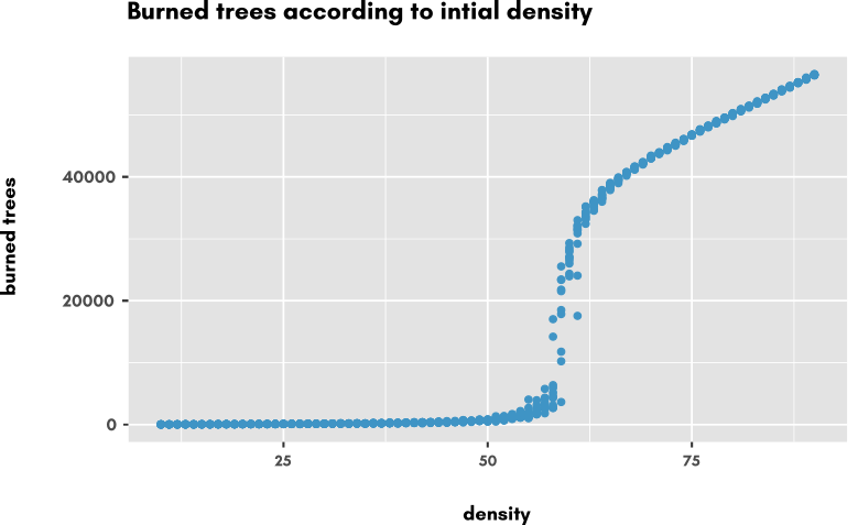
The change of regime clearly appears between 50% and 75% percent density, so we are going to take a closer look at this domain: we change the exploration task to have the density taken from 50% to 75% by step of 0.1%, still with 10 replications:
This gives us the following scatter plot, where we added an "estimator" (or predictor) curve (geom_smooth() from ggplot2 R library to be precise) that acts like a floating estimator in the collection of points, giving the statistical tendency of the Y-Axis values of points along the X-axis.

That's pretty cool already ! The estimator gives us a nice sigmoïd shape on which we could find the mid point, the steepness of the curve and so on, to better characterize the phenomenon.
Fire.nlogo model is a simple, one-parameter, simulation model that simulates fire propagation.
This model features a threshold value in its unique parameter domain, below which fire fails to burn the majority
of the forest, and beyond which fire propagates and burn most of it.
We will perform sensitivity analysis to make this change of regime appear.
The Fire model integration has been covered in the NetLogo page of the Model section, so we take it from here.
The former script was already performing a sensitivity Analysis, by varying density from 20 to 80 by step of 10, with 10 replication for each (seed is taken 10 times).
In our case, the quantum of 10 percent is quite coarsed, so we make it 1 percent :
val exploration =
  ExplorationTask(
    (density in (20.0 to 80.0 by 1.0)) x
    (seed in (UniformDistribution[Int]() take 10))
  )
This is the resulting scatterplot of Number of burned trees according to density varying from 20% to 80% by 1% steps.
The change of regime clearly appears between 50% and 75% percent density, so we are going to take a closer look at this domain: we change the exploration task to have the density taken from 50% to 75% by step of 0.1%, still with 10 replications:
val exploration =
  ExplorationTask(
    (density in (50.0 to 75.0 by 0.1)) x
    (seed in (UniformDistribution[Int]() take 10))
  )
This gives us the following scatter plot, where we added an "estimator" (or predictor) curve (geom_smooth() from ggplot2 R library to be precise) that acts like a floating estimator in the collection of points, giving the statistical tendency of the Y-Axis values of points along the X-axis.
Eventually, let's have a look at the stochasticity of the model. Looking at the plot, we see that there is a lot of variation possible, especially in the transition zone, around 60% density. Let's make a final exploration Task to investigate the variation of model outputs for several replications of the same parameterization. We now take densities within [50;70] and take 100 replications for each:
val exploration =
  ExplorationTask(
    (density in (50.0 to 70.0 by 0.1)) x
    (seed in (UniformDistribution[Int]() take 100))
  )
We obtain the following results, displayed as boxplots every percent (but results are obtained for every 0.1% density) to emphasize on the variations.
As we can see, stochasticity has an high effect right in the middle of the transition of regime, reaching maximum at 54%. Another interesting thing to investigate what would be the density from which the fire propagates to the end of the zone (right side of NetLogo World). A slight modification of the model code would do the trick (hint:
any? patches with-max [pxcor] ... would be a good starting point :-) but we let you do it on your own (any successful attempt would win the right to be displayed right here ! )
For completeness sake, here is the R code snippet to produce plots from your results file (RSutdio version 1.0.153, ggplot2 version 2.2.1)
library(ggplot2)
setwd("~/dev/DocOpenMoleSensitivity/")

df <- read.csv("result.csv")
dfzoom <- read.csv("resultZoom.csv")
dfzoomSeed <- read.csv("resultZoomSeed.csv")


#scatterplot
p <- ggplot(df, aes(x=density, y=burned)) +
       geom_point(colour="#4096c5") +
  ggtitle("Burned trees according to initial Density, with predictor curve and booxplots")+
  ylab("burned trees")+
  theme(panel.background = element_rect(fill = "grey90"))
p

#scatter + estimator
pp <- ggplot(dfzoom, aes(x=density, y=burned)) +
  geom_point(colour="#4096c5") +
  geom_smooth(colour="#ff5900")+
  ggtitle("Burned trees according to initial Density, with predictor curve and booxplots")+
  ylab("burned trees")+
  theme(panel.background = element_rect(fill = "grey90"))
pp

#boxplot every percent
ppp <- ggplot(dfzoomSeed, aes(x=density, y=burned, group=density)) +
  geom_boxplot((aes(group = cut_width(density, 1))), outlier.alpha=0.2,colour="#4096c5", outlier.color = "#ff5900")+
  ggtitle("Stochasticity : Boxplots every percent")+
  ylab("burned trees")+
  scale_x_continuous(breaks=seq(50,70,5), minor_breaks = seq(50,70,1))+
  theme(panel.background = element_rect(fill = "grey90"))
ppp
