 Explore with Calibration
Method scores :
The single criterion Calibration method is designed to solve an optimization problem, so unsurprisingly it performs well regarding the optimization grade. Since it's only focused towards discover the best performing individual (parameter set), this method doesn't provide insights about the sensitivity of the model regarding its inputs, as it does not keep full record of the past input samplings leading to the optimal solution.
For the same reason, this method does not intend to cover the input space and the output space and thus does not perform well regarding the input space and output space exploration grades. It does indeed explore input space, but does not keep track of it. Calibration can handle stochasticity, using a specific method.
This method is not sensitive to the dimensionality of the model output space, as it only need a fitness value, which is a single criterion (value). It is, on the contrary, sensitive the input space dimensionality, as the population of potential solutions to evolve can be tremendous, as well as its fitness gradient hardly tractable.
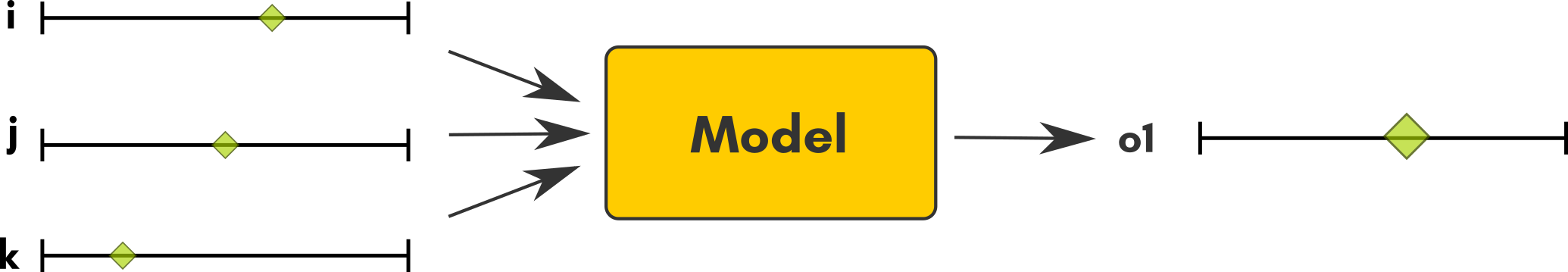
Single criterion calibration answers the question : For a given target value of output o1, what is(are) the parameter set(s) (i, j , k) that produce the closest values of o1 to the target ?
Method scores :
Multi-criteria Calibration method slightly differs from the single criterion version. It suffers the same limitation regarding Input and Output space limitations. However, since it may reveal a Pareto frontier and the underlying tradeoff, it reveals a little bit of the model sensitivity, showing that the model performance regarding a criterion is impacted by its performances regarding the others. This is not genuine sensitivity as in sensitivity analysis, but still, it reveals a variation of your model outputs, which is not bad after all !
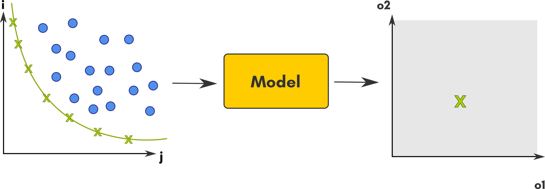
Calibration boils down to minimizing a distance measure between the model output and some data. When there is only a single distance measure considered, it is single criterion calibration. When it there are more than one distance that matter, it is multi-criteria calibration. For example, one may study a prey-predator model and want to find parameter values for which the model reproduce some expected size of both the prey and predator populations.
The single criterion case is simpler, because we can always tell which distance is smaller between any two distances. Thus, we can always select the set of parameter values that is the best.
In the multi-criteria case, it may not always be possible to tell which simulation output has the smallest distance to the data. For example, consider a pair (d1, d2) that represents the differences between the model output and the data for the prey population size (d1) and the predator population size (d2). Two pairs such as (10, 50) and (50, 10) each have one element smaller than the other and one bigger. There is no natural way to tell which pair represents the smaller distance between the model and the data. Thus, in the multi-criteria case, we keep all the parameter sets (e.g. {(i1, j1, k1), (i2, j2, k2), ...}) which yield distances (e.g. {(d11, d21), (d12, d22), ...}) for which we cannot find another parameter set that yields smaller distances for all the distances considered. The set of all these parameter sets is called the Pareto-front.
mu: the population size,genome: a list of the model parameters and their respective intervals,objectives: a list of the distance measures (which in the single criterion case will contain only one measure)
You will also need a evolutionary scheme to drive the evolution and can use the SteadyStateEvolution scheme. it takes the following parameters:
algorithm: the nsga2 algorithm defining the evolution,evaluation: the OpenMOLE task that runs the simulation,parallelism: the number of simulations that will be run in parallel,termination: the total number of evaluations (execution of the task passed to the parameter "evaluation") to be executed
In your OpenMOLE script, the NSGA2 algorithm and SteadyStateEvolution scheme are used like so:
val nsga2 =
  NSGA2(
    mu = 50,
    genome = Seq(
      param1 in (0.0, 99.0),
      param2 in (0.0, 99.0)),
    objectives = Seq(distance1, distance2)
  )

val evolution =
  SteadyStateEvolution(
    algorithm = nsga2,
    evaluation = modelTask,
    parallelism = 10,
    termination = 100
  )
param1 and param2 are input of the modelTask, and distance1 and distance2 are its outputs.
